Distribution Function

Definitions

1. A discrete probability distribution is a table (or a formula) listing all possible values that a discrete variable can take on, together with the associated probabilities.
2. The function f(x) is called a probability density function for the continuous random variable X where the total area under the curve bounded by the x-axis is equal to $\displaystyle{1}$. i.e.

$\displaystyle{\int_{{-\infty}}^{\infty}} f{{\left({x}\right)}}{\left.{d}{x}\right.}={1}$

The area under the curve between any two ordinates x = a and x = b is the probability that X lies between a and b.

$\displaystyle{\int_{{a}}^{{b}}} f{{\left({x}\right)}}{\left.{d}{x}\right.}={P}{\left({a}\le{X}\le{b}\right)}$

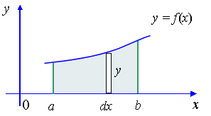
Case 1: Curves which are entirely above the x-axis.

The curve y = f(x), completely above x-axis. Shows a "typical" rectangle, Δx wide and y high.

In this case, we find the area by simply finding the integral:

$\displaystyle\text{Area}={\int_{{a}}^{{b}}} f{{\left({x}\right)}}{\left.{d}{x}\right.}$

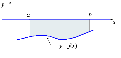
Case 2: Curves which are entirely below the x-axis

We consider the case where the curve is below the $\displaystyle{x}$-axis for the range of $\displaystyle{x}$ values being considered.

In this case, the integral gives a negative number. We need to take the absolute valueof this to find our area:

$\displaystyle\text{Area}={\left|{\int_{{a}}^{{b}}} f{{\left({x}\right)}}{\left.{d}{x}\right.}\right|}$

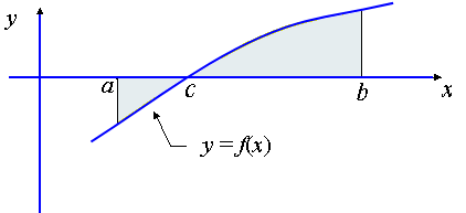
Case 3: Part of the curve is below the x-axis, part of it is above the x-axis

In this case, we have to sum the individual parts, taking the absolute value for the section where the curve is below the $\displaystyle{x}$-axis (from $\displaystyle{x}={a}$ to $\displaystyle{x}={c}$).

$\displaystyle\text{Area}={\left|{\int_{{a}}^{{c}}} f{{\left({x}\right)}}{\left.{d}{x}\right.}\right|}+{\int_{{c}}^{{b}}} f{{\left({x}\right)}}{\left.{d}{x}\right.}$

Summary (so far)

In each of Case 1, Case 2 and Case 3, we are summing elements left to right, like this:

We are (effectively) finding the area by horizontally adding the areas of the rectangles, width $\displaystyle{\left.{d}{x}\right.}$ and heights $\displaystyle{y}$ (which we find by substituting values of $\displaystyle{x}$ into $\displaystyle f{{\left({x}\right)}}$).

So

$\displaystyle{A}={\int_{{a}}^{{b}}} f{{\left({x}\right)}}{\left.{d}{x}\right.}$

(with absolute value signs where necessary, if the curve goes under the $\displaystyle{x}$-axis).

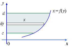
Case 4: Certain curves are much easier to sum vertically

In some cases, it is easier to find the area if we take vertical sums. Sometimes the only possible way is to sum vertically.

In this case, we find the area is the sum of the rectangles, heights $\displaystyle{x}= f{{\left({y}\right)}}$ and width $\displaystyle{\left.{d}{y}\right.}$.

If we are given $\displaystyle{y}= f{{\left({x}\right)}}$, then we need to re-express this as $\displaystyle{x}= f{{\left({y}\right)}}$ and we need to sum from bottom to top.

So, in case 4 we have:

$\displaystyle{A}={\int_{{c}}^{{d}}} f{{\left({y}\right)}}{\left.{d}{y}\right.}$

Probabilities As Relative Frequency

If an experiment is performed a sufficient number of times, then in the long run, the relative frequency of an event is called the probability of that event occurring.

Example 

Refer to the previous example. The weight of a jar of coffee selected is a continuous random variable. The following table gives the weight in kg of $\displaystyle{100}$ jars recently filled by the machine. It lists the observed values of the continuous random variable and their corresponding frequencies.

Find the probabilities for each weight category.

Weight X	Number of Jars
$\displaystyle{0.900}-{0.925}$	$\displaystyle{1}$
$\displaystyle{0.925}-{0.950}$	$\displaystyle{7}$
$\displaystyle{0.950}-{0.975}$	$\displaystyle{25}$
$\displaystyle{0.975}-{1.000}$	$\displaystyle{32}$
$\displaystyle{1.000}-{1.025}$	$\displaystyle{30}$
$\displaystyle{1.025}-{1.050}$	$\displaystyle{5}$
Total	$\displaystyle{100}$

ANSWER

We simply divide the number of jars in each weight category by 100 to give the probabilities.

Weight X	Number of Jars	Probability P(a ≤ X < b)
0.900 - 0.925	1	0.01
0.925 - 0.950	7	0.07
0.950 - 0.975	25	0.25
0.975 - 1.000	32	0.32
1.000 - 1.025	30	0.30
1.025 - 1.050	5	0.05
Total	100	1.00